mono_t2: Compute a monoexponential T2 map
Contents
- 1. Print mono_t2 information
- 2. Setting model parameters
- 2.a. Create mono_t2 object
- 2.b. Set protocol and options
- 2.b.1 Set protocol the CLI way
- 2.b.2 Set protocol and options the GUI way
- 3. Fit MRI data
- 3.a. Load input data
- 3.b. Execute fitting process
- 3.c. Display FitResults
- 3.d. Save fit results
- 3.e. Re-use or share fit configuration files
- 4. Simulations
- 4.a. Single Voxel Curve
- 4.b. Sensitivity Analysis
- 5. Notes
- 5.a. Notes specific to mono_t2
- 5.a.1 BIDS
- 5.b. Generic notes
- 5.b.1. Batch friendly option and protocol conventions
- 5.b.2 Parallelization
- 6. Citations
% This m-file has been automatically generated using qMRgenBatch(mono_t2)
% for publishing documentation.
% Command Line Interface (CLI) is well-suited for automatization
% purposes and Octave.
%
% Please execute this m-file section by section to get familiar with batch
% processing for mono_t2 on CLI.
%
% Demo files are downloaded into mono_t2_data folder.
%
% Written by: Agah Karakuzu, 2017
% ==============================================================================
1. Print mono_t2 information
qMRinfo('mono_t2');
  mono_t2: Compute a monoexponential T2 map

Assumptions:
Mono-exponential fit

Inputs:
SEdata          Multi-echo spin-echo data, 4D volume with different
echo times in time dimension
(Mask)          Binary mask to accelerate the fitting (OPTIONAL)

Outputs:
T2              Transverse relaxation time [s]
M0              Equilibrium magnetization

Protocol:
TE Array [nbTE]:
[TE1; TE2;...;TEn]     column vector listing the TEs [ms]

Options:
FitType         Linear or Exponential
DropFirstEcho   Link Optionally drop 1st echo because of imperfect refocusing
Offset          Optionally fit for offset parameter to correct for imperfect refocusing

Example of command line usage:
Model = mono_t2;  % Create class from model
Model.Prot.SEData.Mat=[10:10:320]'; %Protocol: 32 echo times
data = struct;  % Create data structure
data.SEData = load_nii_data('SEData.nii.gz');
FitResults = FitData(data,Model); %fit data
FitResultsSave_mat(FitResults);

Reference work for DropFirstEcho and Offset options:
https://www.ncbi.nlm.nih.gov/pubmed/26678918

Reference page in Doc Center
doc mono_t2
2. Setting model parameters
2.a. Create mono_t2 object
Model = mono_t2;
2.b. Set protocol and options
Protocol: MRI acquisition parameters that are accounted for by the respective model.
For example: TE, TR, FA FieldStrength. The assigned protocol values are subjected to a sanity check to ensure that they are in agreement with the data attributes.
Options: Fitting preferences that are left at user's discretion.
For example: linear fit, exponential fit, drop first echo.
2.b.1 Set protocol the CLI way
If you are using Octave, or would like to serialize your operations any without GUI involvement, you can assign protocol directly in CLI:
EchoTime  = [12.8000; 25.6000; 38.4000; 51.2000; 64.0000; 76.8000; 89.6000; 102.4000; 115.2000; 128.0000; 140.8000; 153.6000; 166.4000; 179.2000; 192.0000; 204.8000; 217.6000; 230.4000; 243.2000; 256.0000; 268.8000; 281.6000; 294.4000; 307.2000; 320.0000; 332.8000; 345.6000; 358.4000; 371.2000; 384.0000];
% EchoTime (ms) is a vector of [30X1]
Model.Prot.SEdata.Mat = [ EchoTime ];
See the generic notes section below for further information.
2.b.2 Set protocol and options the GUI way
The following command opens a panel to set protocol and options (if GUI is available to the user):
Model = Custom_OptionsGUI(Model);
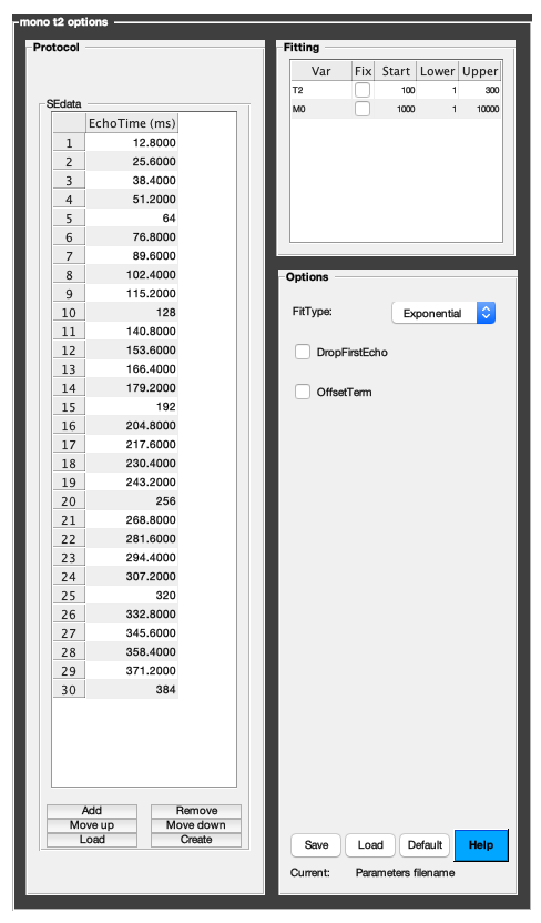
If available, you need to close this panel for the remaining of the script to proceed.
Using this panel, you can save qMRLab protocol files that can be used in both interfaces. See the generic notes section below for details.
3. Fit MRI data
3.a. Load input data
This section shows how you can load data into a(n) mono_t2 object.
- At the CLI level, qMRLab accepts structs containing (double) data in the fields named in accordance with a qMRLab model.
See the generic notes section below for BIDS compatible wrappers and scalable
qMRLab workflows.
%          |- mono_t2 object needs 2 data input(s) to be assigned:
%          |-   SEdata
%          |-   Mask

data = struct();
% SEdata.nii.gz contains [260  320    1   30] data.
data.SEdata=double(load_nii_data('mono_t2_data/SEdata.nii.gz'));
% Mask.nii.gz contains [260  320] data.
data.Mask=double(load_nii_data('mono_t2_data/Mask.nii.gz'));
3.b. Execute fitting process
This section will fit the loaded data.
FitResults = FitData(data,Model,0);
Visit the generic notes section below for instructions to accelerate fitting by
parallelization using ParFitData.
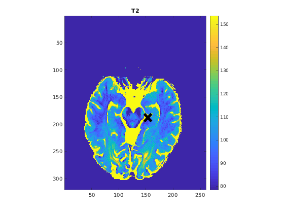
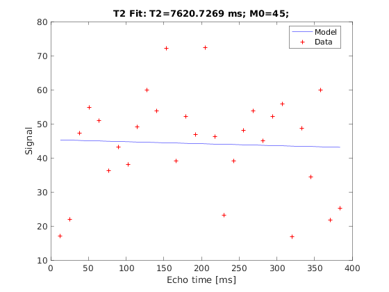
3.c. Display FitResults
You can display the current outputs by:
qMRshowOutput(FitResults,data,Model);
A representative fit curve will be plotted if available.
To render images in this page, we will load the fit results that had been saved before. You can skip the following code block;
% Load FitResults that comes with the example dataset.
FitResults_old = load('FitResults/FitResults.mat');
qMRshowOutput(FitResults_old,data,Model);
3.d. Save fit results
Outputs can be saved as *.nii.(gz) if NIfTI inputs are available:
% Generic function call to save nifti outputs
FitResultsSave_nii(FitResults, 'reference/nifti/file.nii.(gz)');
If not, FitResults.mat file can be saved. This file contains all the outputs as workspace variables:
% Generic function call to save FitResults.mat
FitResultsSave_mat(FitResults);
FitResults.mat files can be loaded to qMRLab GUI for visualization and ROI
analyses.
The section below will be dynamically generated in accordance with the example data format (mat or nii). You can substitute FitResults_old with FitResults if you executed the fitting using example dataset for this model in section 3.b..
FitResultsSave_nii(FitResults_old, 'mono_t2_data/SEdata.nii.gz');
3.e. Re-use or share fit configuration files
qMRLab's fit configuration files (mono_t2_Demo.qmrlab.mat) store all the options and protocol in relation to the used model and the release version.
*.qmrlab.mat files can be easily shared with collaborators to allow them fit their own
data or run simulations using identical option and protocol configurations.
Model.saveObj('my_mono_t2_config.qmrlab.mat');
4. Simulations
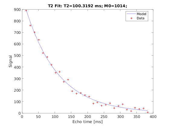
4.a. Single Voxel Curve
Simulates single voxel curves
      x = struct;
x.T2 = 100;
x.M0 = 1000;
Opt.SNR = 50;
% run simulation
figure('Name','Single Voxel Curve Simulation');
FitResult = Model.Sim_Single_Voxel_Curve(x,Opt);
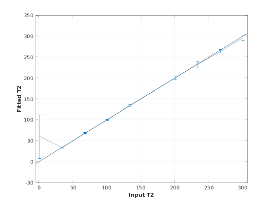
4.b. Sensitivity Analysis
Simulates sensitivity to fitted parameters
T2 M0
      OptTable.st = [1e+02         1e+03]; % nominal values
OptTable.fx = [0             1]; %vary T2...
OptTable.lb = [1             1]; %...from 1
OptTable.ub = [3e+02         1e+04]; %...to 300
Opt.SNR = 50;
Opt.Nofrun = 5;
% run simulation
SimResults = Model.Sim_Sensitivity_Analysis(OptTable,Opt);
figure('Name','Sensitivity Analysis');
SimVaryPlot(SimResults, 'T2' ,'T2' );
5. Notes
5.a. Notes specific to mono_t2
5.a.1 BIDS
![]()
|== sub-01/
|~~~~~~ anat/
|---------- sub-01_echo-1_MESE.json
|---------- sub-01_echo-1_MESE.nii.gz
|---------- sub-01_echo-2_MESE.json
|---------- sub-01_echo-2_MESE.nii.gz
|---------- .
|---------- .
|---------- sub-01_echo-N_MESE.json
|---------- sub-01_echo-N_MESE.nii.gz
|
|== derivatives/
|~~~~~~ qMRLab/
|---------- dataset_description.json
|~~~~~~~~~~ sub-01/anat/
|-------------- sub-01_T2map.nii.gz
|-------------- sub-01_T2map.json
|-------------- sub-01_M0map.nii.gz
|-------------- sub-01_M0map.json
For further information, please visit BIDS qMRI Appendix.
5.b. Generic notes
5.b.1. Batch friendly option and protocol conventions
If you would like to load a desired set of options / protocols programatically, you can use *.qmrlab.mat files. To save a configuration from the protocol panel of mono_t2, first open the respective panel by running the following command in your MATLAB command window (MATLAB only):
Custom_OptionsGUI(mono_t2);
In this panel, you can arrange available options and protocols according to your needs, then click the save button to save my_mono_t2.qmrlab.mat file. This file can be later loaded into a mono_t2 object in batch by:
Model = mono_t2;
Model = Model.loadObj('my_mono_t2.qmrlab.mat');
Model.loadObj('my_mono_t2.qmrlab.mat') call won't update the fields in the Model object, unless the output is assigned to the object as shown above. This compromise on convenience is to retain Octave CLI compatibility.
If you don't have MATLAB, hence cannot access the GUI, two alternatives are available to populate options:
- Use qmrlab/mcrgui:latest Docker image to access GUI. The instructions are available here.
- Set options and protocols in CLI:
- List available option fields using tab completion in Octave's command prompt (or window)
Model = mono_t2;
Model.option. % click the tab button on your keyboard and list the available fields.
- Assign the desired field. For example, for a mono_t2 object:
Model = mono_t2;
Model.options.DropFirstEcho = true;
Model.options.OffsetTerm = false;
Some option fields may be mutually exclusive or interdependent. Such cases are handled by the GUI options panel; however, not exposed to the CLI. Therefore, manual CLI options assignments may be challenging for some involved methods such as qmt_spgr or qsm_sb. If above options are not working for you and you cannot infer how to set options solely in batch, please feel free to open an issue in qMRLab and request the protocol file you need.
Similarly, in CLI, you can inspect and assign the protocols:
Model = mono_t2;
Model.Prot. % click the tab button on your keyboard and list the available fields.
Each protocol field has two subfields of Format and Mat. The first one is a cell indicating the name of the protocol parameter (such as EchoTime (ms)) and the latter one contains the respective values (such as 30 x 1 double array containing EchoTimes).
The default Mat protocol values are set according to the example datasets served via OSF.
5.b.2 Parallelization
Beginning from release 2.5.0, you can accelerate fitting for the voxelwise models using parallelization.
Available in MATLAB only. Requires parallel processing toolbox.
In CLI, you can perform parallel fitting by:
parpool();
FitResults = ParFitData(data,Model);
If a parpool exists, the ParFitData will use it. If not, a new pool will be created using the local profile. By default, ParFitData saves outputs automatically every 5 minutes. You can disable this feature by:
FitResults = ParFitData(data, Model, 'AutosaveEnabled', false);
Alternatively, you can change the autosave interval (min 1 min) by:
FitResults = ParFitData(data,Model,'AutoSaveInterval',10);
If something went wrong during the fitting (e.g. your computer had to be restarted), you can recover the autosaved data by:
FitResults = ParFitData(data,Model,'RecoverDirectory','/ParFitTempResults_*/folder/from/the/previous/session');
GUI users will be prompted a question about whether they would like to use parallelization after clicking the Fit Data button, if the conditions are met. When called from GUI, ParFitData will be run with default options:
- Save temporary results every 5 minutes or whenever a chunk has finished processing
- Split data into chunks with a granularity factor of 3
- Do not remove temporary fit results upon completion
For further information:
help ParFitData
The default parallelization options can be changed in the preferences.json file located at the root qMRLab directory.
6. Citations
qMRLab JOSS article
Karakuzu A., Boudreau M., Duval T.,Boshkovski T., Leppert I.R., Cabana J.F., Gagnon I., Beliveau P., Pike G.B., Cohen-Adad J., Stikov N. (2020), qMRLab: Quantitative MRI analysis, under one umbrella 10.21105/joss.02343
Reference article for mono_t2
Quantitative MRI, under one umbrella.
NeuroPoly Lab, Montreal, Canada