Graphical User Interface (GUI)
This section describes the various features and functionality of the user interface.
1. Startup
Launch matlab from the qMRLab folder. Then load the default setup by typing:
startup
Then open the GUI by typing:
qMRLab
2. Layout
When you first launch qMRLab, you will be presented with a blank interface. The interface consists of three columns, or panels. On the left, you have the Menu panel, in the center you have the Main panel, and on the right, in a separate floating window, you have the Options panel.
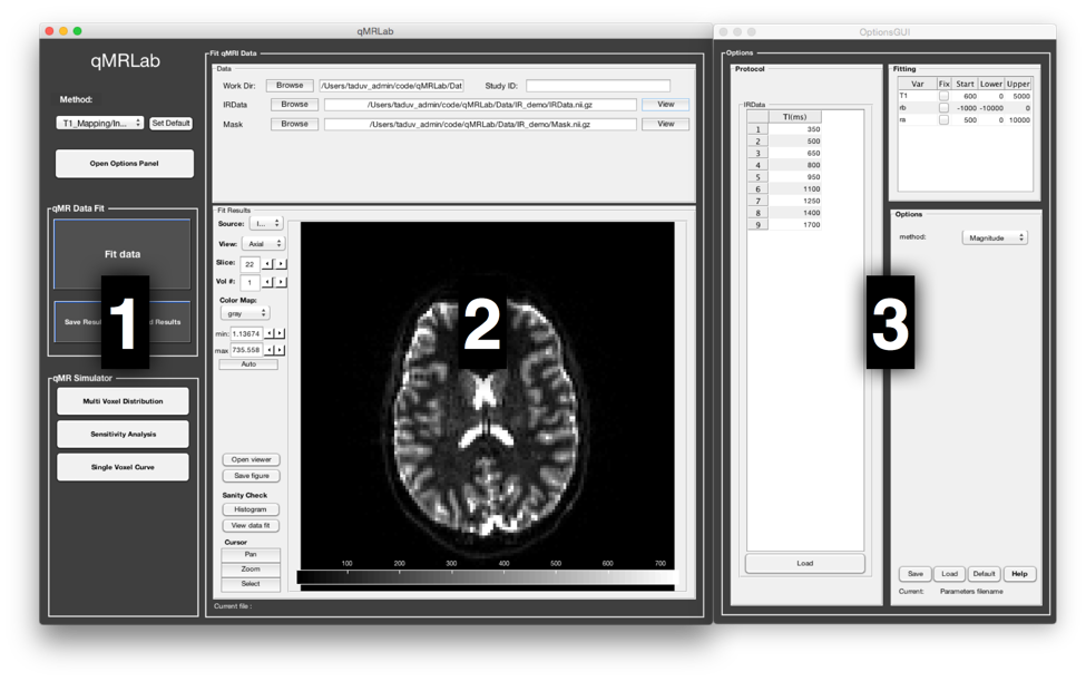
Default interface with 3 panels: (1) Menu, (2) Main and (3) floating Options
2.2 Main Panel
The Main panel is where you can load your data files for fitting and for viewing the resulting parameters maps. This panel changes correspondingly to the Method selected in the Menu panel.
2.3 Options Panel
This is where you can set up all the parameters that are related to the simulation, the fitting and the protocol. The Options panel is displayed in a separate window than the Menu panel or Main panel. This is because each qMR acquisition method has its own particular options, and this window needs to be changed correspondingly. It can also be closed at any time, if it is not currently needed, to provide for a simpler interface. The Options panel consists of three sub-panels: Protocol, Fitting, and Options. At the bottom of all these sub-panels you will find buttons to Reset the changes you made, Save the current settings as a .mat file, Load a .mat file of settings, or go back to the Default settings. Refer to section 6. Options Panel for more information.
2.3.1 Protocol
Here you define the acquisition protocol that you wish to use for simulation, or in the case of data fitting, the protocol you used to acquire the data. See 6.1 Protocol for more information.
2.3.2 Fitting
This is where you set up your fitting options. The fit parameters table lists all the variables that are available for fitting in the current method, a tick box to select which variables are to be held fixed, a starting value and lower/upper bounds. Note that some methods do not have fitting procedures, this table is empty in this case. Depending on the method, additional options may be available. See 6.2. Fitting for more information.
2.3.3 Options
This is where you set up all the options related to the simulations. Depending on the qMR method, different sets of options are available (e.g. the fitting procedure, assumptions of the model, etc). More info in 6.3. Options.
3. Data Viewer
The viewer allows you to navigate through your (up tp) 5D dataset easily using arrows:

Use mouse controls to display your volume:
| Middle (shift+) Click and drag: | |
|---|---|
| Zoom in/out | |
| Left Click and drag: | |
| Contrast/Brightness | |
| Right (ctrl+) Click and drag: | |
| Pan | |
| Scroll wheel: | Change slice |

The viewer provides ROI tools to create and modify a multi-label mask that is overlaid on the image.
The Mask in the file browser is loaded automatically, you can delete it using right click on the button label 1.
The mask can be hidden/shown using the checkbox on the top (or use spacebar)… make sure the mask is toggle on when you draw it!
The mask can have 5 different labels (1-5). Select the label on which you want to operate. One voxel can be attributed only one label (no overlaps between labels). The locker button prevents any modification and overwrite to labels that are not selected.
ROI tools such as square or polygon can be converted to mask (right click on an ROI object) and conversely (mask2poly button).
Statistics on each label (e.g. volume, mean intensity) can be obtained with mouse over the label number.
Brush tool controls:
| Middle click and drag: | |
|---|---|
| Change brush diameter | |
| Right click: | erase |
| double click: | (smart brush only) Toggle between bright or dark segmentation |
Polygon tool controls:
| Click on a line: | |
|---|---|
| add a button | |
| Double click on a point: | |
| toggle between a line and a curve | |
| Middle click on a point: | |
| delete this intermediary point | |
4. Data Fitting
qMRLab provides a convenient interface to fit your data and visualize the parameters maps. To ensure that the results are successful, you’ll need to define the appropriate protocol, as it was used for data acquisition, and to format your qMR data in the way qMRLab expects it to be.
4.1 Data format
Currently supported file types are .mat and .nii files. Your files should respect the following:
- For .mat files, the name of the file can be anything, but the array it contains should be named appropriately. The list of input names is case sensitive and is specified at the top of the
Datadialog box. For example, for a qMT SPGR experiment,MTdata(for the actual MT data array) or R1map / B1map / B0map / Mask respectively for a R1 / B1 / B0 or Mask file.

Example of list of inputs for qMT SPGR experiment
- Each model will expect a different format of inputs, but in general, for single slice (2D) imaging, the main data is a 3D array with size [nx, ny, ndata], where nx/ny is the number of voxels in the x/y direction, and ndata is the number of data points for each voxel. For volume imaging (3D), data is a 4D array with size [nx, ny, nz, ndata], where nx/ny/ndata are as above, and nz is the number of voxels (or slices) in the z direction (e.g. in this example MTdata would have several datapoints per voxel).
- Other files (e.g. in this example R1map / B1map / B0map / Mask) are formatted as [nx, ny, nz].
For a more detailed description of the format required for each input, type this in the maltab window:
help Modelname
where Modelname is name of the available models (e.g. in this example help SPGR). Alternatively, in the Options panel, you can press on the Help button
4.2 Fitting Procedure
4.2.1 Single voxel
This is useful when you want to preview the fit of a single voxel (note this option is only available on voxelwise computations)
- Select the acquisition method of your data using the ‘Method’ drop-down menu in the
Menupanel. - In the
Menupanel, in theFit qMR datapanel, enter your study ID in theStudy IDbox (optional). - Load your data by clicking the browse button beside the
Data:line, or enter the full file path to it in the textbox. - You can view any of these maps by clicking its
Viewbutton.

Example of viewing option, in this case R1map used for qMT SPGR
- Define or load the appropriate protocol in the Options panel (see 6.1 Protocol for details).
- Define your fitting options in the Options panel (see 6.2. Fitting for details).
- You can preview the fitted curve for a selected voxel by using the
View Data Fitbutton. Make sure a dataset is loaded by clickingViewbeside the data file field - Click
Selectbutton in theCursorsection to activate voxel selection mode, select a voxel to preview and clickView Data Fit. You can now see the fitted curve and the parameters computed for that voxel.
Example of fitting in 1 voxel, which was selected with the cursor on the image.
4.2.2 Whole dataset
Follow steps 1-6 above, then
- In the Menu panel, click on
Fit datato start the fitting process. - Once the fitting is done, a temporary file will be saved in the ‘FitResults’ subfolder of the current working directory. You can save the current fit results elsewhere by clicking
Save Resultsin the ‘qMR data fit’ section of the Menu panel. - Use the controls in the
Fit Resultssection to visualize the results (ssee 4.3 Viewing the fit results for details).
4.3 Viewing the fit results
Once you have finished fitting your qMR data, or when you load previously saved fit results by clicking Load Results in the qMR data fit section of the Menu panel, the maps will be displayed in the Fit Results section. Use controls on the left side of the figure to navigate the maps:
- Source: select the parameter map to display
- View: select the side from which to view the data (available only on 3D maps)
- Slice: navigate through the z direction of the current view (available only on 3D maps)
- Color Map: choose the color scheme to use from a set of pre-defined Malab colormaps
- Range: Control the colormap min/max values. Clicking ‘Auto’ will set the min/max values using the min/max of the currently displayed image. Top textbox/slider allows you to manually set the Min value, while bottom textbox/slider are for the Max value
- Open viewer: open the current data in an external viewer to display simultaneous axial/sagittal/coronal views.
- Save figure: save the current figure
- Histogram: open a new window with an histogram of the voxels in the currently selected slice (note that zooming in on a particular section while still produce an histogram of the full slice)
- View data fit: display raw data + fitted curve of the currently selected voxel (use ‘Cursor’ button to activate voxel selection mode).
- Pan: change the cursor mode to ‘Pan’. Click and hold inside the figure to move around. Double click inside the figure to reset view. Clicking again the Pan button will turn off pan mode.
- Zoom: change the cursor mode to ‘Zoom’. Click and hold inside the figure to draw a region to zoom in on. Double click inside the figure to reset view. Clicking again the Zoom button will turn off zoom mode.
- Select: change the cursor mode to ‘Data Cursor’. Click on a voxel to display info (X/Y is the position of the voxel, index is the value of the map at this point, RGB is the mapped color code).
5. Simulation
5.1. Single Voxel Curve
The Single Voxel Curve simulation interface allows you to simulate qMR data for the defined parameters and protocol. Once the simulation is done, you can also rapidly test the effect of changing fitting options without having to run the simulation again. It is the fastest way to evaluate various acquisition protocols and the performance of the model and fitting options. A plot of the fitted curve over the actual data will be displayed, and the resulting fitted parameters are compared to the input parameters.
- Select the acquisition method of your qMR data using the ‘Method’ drop-down menu in the Menu panel.
- In the Menu panel, click on Single Voxel Curve to display the interface in the Main panel.
- Using the Options panel, define or load the protocol you wish to use (see section 5.1).
- Using the Options panel, define or load your initial fitting options (see section 5.2).
- Using the
Optionspanel, define or load your simulation parameters (see section 5.3). - In the
Menupanel, click on the bigSimulate databutton. A progress bar will appear to show the progression of the simulation. ClickingCancelin the progress bar window will stop the current simulation. - Once the simulation is done, the results are displayed in the
Mainpanel. - If you want to see the effect of changing fitting options, use the Options panel to make your changes. Then, in the
Mainpanel inside the ‘Simulation Fit Results’ panel, click onUpdate Fit. Clicking this button without changing fitting options will also generate a new noisy data distribution and recalculate the fitted curve. - Once the fitting is done, a temporary file (SimCurveTempResults) will be saved in the ‘SimResults’ subfolder of the current active method (e.g. qMTLab/SPGR/SimResults/). You can save the current simulation results by clicking
Save Resultsin theqMR Data Simulator fitsection of the Menu panel. You can later load it using theLoad Resultsbutton.

Example result of simulation in 1 voxel. Remember to set options in ‘Options’ panel
5.2. Sensitivity Analysis
The Sensitivity Analysis simulation allows you to systematically vary one parameter, over a defined range and number of points, while keeping the others fixed. For each simulated data point, noise is added with a given SNR, and the fit is run multiple times while adding gaussian noise. This allows you to evaluate the variance of the fit at each point. When the simulation is done, a plot shows any variable input parameters as the independent variable, as well as the mean values and variance of any fitted parameters.
- Select the acquisition method of your data using the ‘Method’ drop-down menu in the Menu panel.
- In the Menu panel, click on Sensitivity Analysis to display the interface in the Main panel.
- Using the Options panel, define or load the protocol you wish to use (see section 5.1).
- Using the Options panel, define or load your fitting options (see section 5.2).
- Using the Options panel, define or load your simulation parameters (see section 5.3). The parameters defined here are used as the fixed parameters values as one parameter at a time is systematically varied during the simulation process.
- In the Main panel, use the ‘Parameters variation’ table to define your analysis settings. Select the parameters that are to be varied by setting a mark in the appropriate checkbox, set the minimum and maximum values for this parameter under the column ‘Min’ and ‘Max’, and the size of the incrementing step under ‘Step’. Set the number of times you want to add noise and fit for each data point by entering an integer value in the ‘# of runs’ box. These settings can be saved, retrieved or reset to their initial settings using the ‘Save’, ‘Load’ and ‘Reset’ buttons respectively.
- In the Menu panel, click on the big Simulate data button. A progress bar will appear to show the progression of the simulation. Clicking Cancel in the progress bar window will stop the current simulation.
- Once the simulation is done, the results are displayed in the ‘Plot Results’ section in the Main panel. Using the ‘x axis’ and ‘y axis’ dropdown menu, you can change the independent/dependant parameters respectively. The parameters that have been varied will be available under the ‘x axis’ menu, while all the model parameters will be available under the ‘y axis’ menu.
- A temporary file (SimVaryTempResults) will be saved in the ‘SimResults’ subfolder of the current active method (e.g. qMTLab/SPGR/SimResults/). You can save the current simulation results by clicking Save Results in the ‘qMT Data Simulator fit’ section of the Menu panel. You can later load it using the Load Results button.
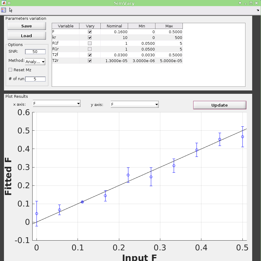
Example of sensitivity analysis of the F parameter for qMT
5.3. Multi Voxel Distribution
The Multi Voxel Distribution is a tool to simulate any number of voxels, where any combination of parameters are allowed to be varied simultaneously. You can choose how many voxels to simulate and which parameters are to be normally distributed, with its mean value and variance. The results can be displayed in a number of ways such as distribution histograms, scatter plots of input vs fitted parameters, error histograms, etc.
- Select the acquisition method of your qMR data using the ‘Method’ drop-down menu in the Menu panel.
- In the Menu panel, click on Multi Voxel Distribution to display the interface in the Main panel.
- Using the Options panel, define or load the protocol you wish to use (see section 5.1).
- Using the Options panel, define or load your fitting options (see section 5.2).
- Using the Options panel, define or load your simulation parameters (see section 5.3). The parameters defined here are used as the fixed parameters values for parameters that are not selected to be varied.
- In the Main panel, use the ‘Parameters distribution’ table to define your distribution settings. Select the parameters that are to be varied by setting a mark in the appropriate checkbox, set the mean and standard deviation values for this parameter under the column ‘Mean’ and ‘Std’ respectively. Set the number of voxels you want to simulate by entering an integer value in the ‘# of voxels’ box. These settings can be saved, retrieved or reset to their initial settings using the Save, Load and Reset buttons respectively.
- Click on Get Parameters in the ‘Parameters distribution’ section to generate a set of normally distributed parameters using the current settings. You can look at the distribution in the ‘Plot Results’ section, by choosing ‘Input parameters’ under the ‘Plot type’ dropdown menu. Select the parameters you want to look at with the ‘x axis’ dropdown menu. You can generate a new set of random values by clicking on the Get Parameters button again.
- In the Menu panel, click on the big Simulate data button. A progress bar will appear to show the progression of the simulation. Clicking Cancel in the progress bar window will stop the current simulation.
- Once the simulation is done, the results are displayed in the ‘Plot Results’ section in the Main panel. Using the ‘Plot type’ dropdown menu, choose what plot you want to view. Plot types are defined below.
- A temporary file (SimRndTempResults) will be saved in the ‘SimResults’ subfolder of the current active method (e.g. qMTLab/SPGR/SimResults/). You can save the current simulation results by clicking ‘Save Results’ in the ‘qMT Data Simulator fit’ section of the Menu panel. You can later load it using the ‘Load Results’ button.
Plot types
Different plot types are available to analyze your simulation results. Depending on the plot type, available selections under ‘x axis’ and ‘y axis’ dropdown menus will change accordingly.
- Input parameters: Histogram of initial input parameters distribution.
- Fit results: Histogram of fitted parameters distribution.
- Input vs. Fit: Scatter plot of input parameter value vs fitted value.
- Error: Histogram of the error distribution. Error is defined as: Fit-Input
- Pct error: Histogram of the percentage error distribution. Percentage error is defined as: 100×(Fit-Input)/Input
- MPE: Bar graph of the mean percentage error, defined as: 100/n ∑((Fit-Input)/Input), where n is the number of simulated voxels.
- RMSE: Bar graph of the root mean squared error, defined as: √(1/n∑(Fit-Input)^2), where n is the number of simulated voxels.
- NRMSE: Bar graph of the normalized root mean squared error, defined as RMSE/(max(Input)-min(Input)) , where max(Input) is the maximum value in the input parameter distribution, and min(Input) is the minimum value.
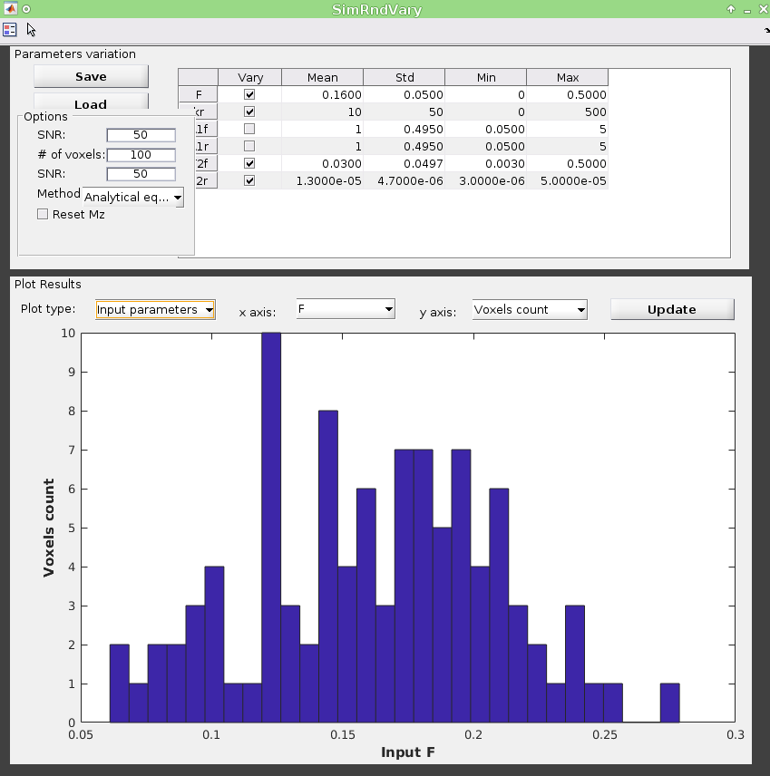
Example of MultiVoxel Distribution (option: Input parameters)
6. Options Panel
Each qMR acquisition method has its own particular options for simulation, protocol and fitting. These options can be modified by using the Options panel. The Options panel consists of three sub-panels of options: ‘Protocol’, ‘Fitting’ and ‘Options’. At the bottom of all these sub-panels you will find buttons to Reset the changes you made, Save the current settings as a .mat file, Load a .mat file of settings, or go back to the Default settings. The Help button will open the help for the particular model.
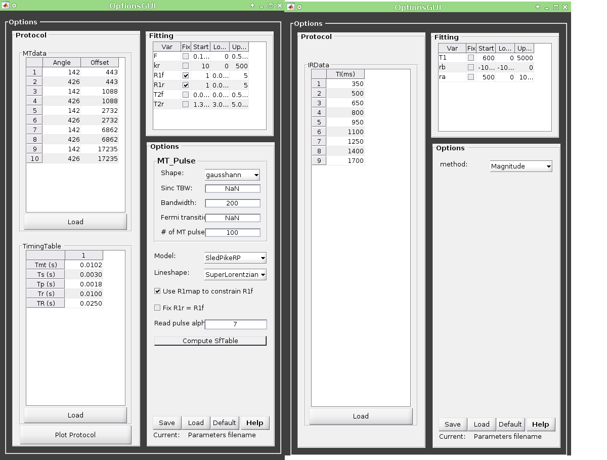
Example of Options panel for qMT SPGR and Inversion Recovery
6.1 Protocol
The ‘Protocol’ panel is where you define all options relating to the acquisition sequence. These options are specific for each method. For all methods, you will find (at the top of the protocol panel) input text fields corresponding to the independent variables. You will need to load a previously saved text (.txt) file with the required options and format by using the Load button. Press the Help button in this panel to see the format expected by each of the models in the Protocol section
For example, the vfa_t1 model is expecting
- Protocol
- VFAData Array [nbFA x 2]:
- [FA1 TR1; FA2 TR2;…] flip angle [degrees] TR [s]
Which means a text file where each row is a different flip angle, 1st column is the flip angle in degrees, 2nd is the TR in sec, e.g.:
3 0.015
20 0.015
6.2. Fitting
The ‘Fitting’ panel is where you determine the upper, lower and starting points of your parameters. You can also select which parameters should be kept fixed for the fitting.
6.3. Options
The ‘Options’ panel is where you specify the properties of the model and the fitting. For example, the assumptions/type of model (e.g. for SPGR, the SledPikeRP or Yarnykh model), type of images (magnitude or magnitude/phase for Inversion Recovery), etc.
7. Tutorial
See the video here: